
目录
介绍
回归模型
线性回归
局部加权线性回归
岭回归
套索(Lasso)回归
逐步线性回归
结论与分析
可访问 实现机器学习的循序渐进指南系列汇总,获取本系列完成文章列表。
介绍通常存在变量之间的关系。实际上,这种关系可以分为两类,即确定关系和不确定关系。确定性关系可以用函数表示。确定性关系也称为相关性,可以用回归分析进行研究。
通常,线性回归模型是:

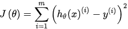
最优化![]() 可以通过最小损失函数来确定:
可以通过最小损失函数来确定:
线性回归包括线性回归,局部加权线性回归,岭回归,套索回归和逐步线性回归。
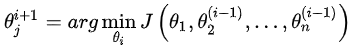
线性回归线性回归的参数![]() 可以通过梯度下降法或正则表达式计算。由于梯度下降法已经在实现机器学习的循序渐进指南IV——逻辑回归中引入,因此我们在本文中介绍具有正则表达式的解决方案。
可以通过梯度下降法或正则表达式计算。由于梯度下降法已经在实现机器学习的循序渐进指南IV——逻辑回归中引入,因此我们在本文中介绍具有正则表达式的解决方案。
首先,计算损失函数的导数:

然后,使导数等于0,我们可以得到:
![]()
最后,![]() 是:
是:
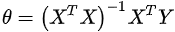
其中X是训练数据,Y是相应的标签。线性回归的代码如下所示:
def standardLinearRegression(self, x, y):
    if self.norm_type == "Standardization":
        x = preProcess.Standardization(x)
    else:
        x = preProcess.Normalization(x)

    xTx = np.dot(x.T, x)
    if np.linalg.det(xTx) == 0:   # calculate the Determinant of xTx
        print("Error: Singluar Matrix !")
        return
    w = np.dot(np.linalg.inv(xTx), np.dot(x.T, y))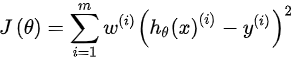
return w使用最小均方误差(MMSE)的无偏估计,它在线性回归中是不合适的。为了解决这个问题,我们在要预测的点周围的点上分配权重。然后,我们对其应用常规回归分析。局部加权线性回归的损失函数是:
像线性回归一样,我们计算损失函数的导数并使其等于0。最优的![]() 是
是
![]()
局部加权线性回归中的权重类似于SVM中的核函数(kernel function),其由下式给出:

局部加权线性回归的代码如下所示:
def LWLinearRegression(self, x, y, sample):
    if self.norm_type == "Standardization":
        x = preProcess.Standardization(x)
    else:
        x = preProcess.Normalization(x)

    sample_num = len(x)
    weights = np.eye(sample_num)
    for i in range(sample_num):
        diff = sample - x[i, :]
        weights[i, i] = np.exp(np.dot(diff, diff.T)/(-2 * self.k ** 2))
    xTx = np.dot(x.T, np.dot(weights, x))
    if np.linalg.det(xTx) == 0:
        print("Error: Singluar Matrix !")
        return
    result = np.dot(np.linalg.inv(xTx), np.dot(x.T, np.dot(weights, y)))
return np.dot(sample.T, result)如果特征维度大于样本数量,则输入矩阵不是满秩,其逆矩阵不存在。为了解决这个问题,岭回归增加了![]() 到矩阵的非奇异性。实际上,对于岭回归的损失函数,等于加上L2正则化,即:
到矩阵的非奇异性。实际上,对于岭回归的损失函数,等于加上L2正则化,即:

像线性回归一样,我们计算损失函数的导数并使其等于0.最优的![]() 是:
是:

岭回归的代码如下所示:
def ridgeRegression(self, x, y):
    if self.norm_type == "Standardization":
        x = preProcess.Standardization(x)
    else:
        x = preProcess.Normalization(x)

    feature_dim = len(x[0])
    xTx = np.dot(x.T, x)
    matrix = xTx + np.exp(feature_dim)*self.lamda
    if np.linalg.det(xTx) == 0:
        print("Error: Singluar Matrix !")
        return
    w = np.dot(np.linalg.inv(matrix), np.dot(x.T, y))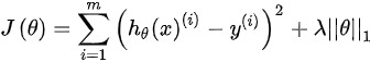
return w与岭回归一样,套索(Lasso)回归在损失函数上加上L1正则化,即:
因为L1正则化包含绝对值表达式,所以损失函数不能在任何地方导出。因此,我们应用坐标下降法(CD)。CD在每次迭代的方向上得到最小值,即
我们可以得到一个封闭的CD解决方案,由下面给出:
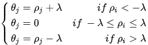
其中:

套索(Lasso)回归的代码如下所示:
def lassoRegression(self, x, y):
    if self.norm_type == "Standardization":
        x = preProcess.Standardization(x)
    else:
        x = preProcess.Normalization(x)

    y = np.expand_dims(y, axis=1)
    sample_num, feataure_dim = np.shape(x)
    w = np.ones([feataure_dim, 1])
    for i in range(self.iterations):
        for j in range(feataure_dim):
            h = np.dot(x[:, 0:j], w[0:j]) + np.dot(x[:, j+1:], w[j+1:])
            w[j] = np.dot(x[:, j], (y - h))
            if j == 0:
                w[j] = 0
            else:
                w[j] = self.softThreshold(w[j])
return w逐步线性回归类似于套索(Lasso)回归,它在每次迭代时应用贪婪算法以获得最小值而不是CD。逐步线性回归在每次迭代时增加或减少一小部分权重。逐步线性回归的代码如下所示:
def forwardstepRegression(self, x, y):
    if self.norm_type == "Standardization":
        x = preProcess.Standardization(x)
    else:
        x = preProcess.Normalization(x)

    sample_num, feature_dim = np.shape(x)
    w = np.zeros([self.iterations, feature_dim])
    best_w = np.zeros([feature_dim, 1])
    for i in range(self.iterations):
        min_error = np.inf
        for j in range(feature_dim):
            for sign in [-1, 1]:
                temp_w = best_w
                temp_w[j] += sign * self.learning_rate
                y_hat = np.dot(x, temp_w)
                error = ((y - y_hat) ** 2).sum()           # MSE
                if error < min_error:                   # save the best parameters
                    min_error = error
                    best_w = temp_w
        w = best_w
return w有许多解决方案可以获得线性回归的最优参数。在本文中,我们仅介绍一些基本算法。最后,让我们将线性回归与Sklearn中的线性回归进行比较,检测性能如下所示:
Sklearn线性回归性能:

我们的线性回归性能:

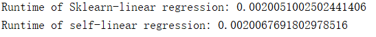
性能看起来很相似。
可以在MachineLearning中找到本文中的相关代码和数据集。
有兴趣的小伙伴可以查看上一篇或者下一篇。
原文地址:https://www.codeproject.com/Articles/5061034/Step-by-Step-Guide-to-Implement-Machine-Learning-6

