qesa Efficient zero-knowledge arguments in the discrete log setting 学习笔记

1. 引言

Hoffmann等人 2019年论文 《Efficient zero-knowledge arguments in the discrete log setting 》。

相应的代码实现可参见：

• https://github.com/crate-crypto/qesa
• https://github.com/emsec/QESA_ZK

总结： 1） 将Bulletproofs中的vector-vector multiplication扩展至了matrix-vector multiplication argument，构建的zero-knowledge argument有： – L M P A s i m p l e Z K LMPA_{simpleZK} LMPAsimpleZK​ 协议：简单的 ∑ s t d \sum_{std} ∑std​ 协议和 L M P A n o Z K LMPA_{noZK} LMPAnoZK​ 协议组合。 – L M P A Z K LMPA_{ZK} LMPAZK​ 协议：区别于Bulletproofs中引入random row vector来实现hiding，本文是通过引入random column vector来实现hiding。（且random column vector 可直接从 random matrix [ h ] [\mathbf{h}] [h] 中逐列获取。） 2） 提出了三种inner product protocol： – I P A n o Z K IPA_{noZK} IPAnoZK​ 协议：实现方式与Bulletproofs类似，无zero-knowledge属性； – I P A a l m Z K IPA_{almZK} IPAalmZK​ 协议：借助kernel guideline来引入特定的随机变量 r ⃗ ′ , r ⃗ ′ ′ \vec{r}',\vec{r}'' r ′,r ′′ 来实现hiding，从而实现zero-knowledge； – Q E S A I n n e r QESA_{Inner} QESAInner​ 协议：通过random linear combination （通过 x ⃗ \vec{x} x 和 s ⃗ ′ \vec{s}' s ′），将多个matrix-vector multiplication转换为 I P A a l m Z K IPA_{almZK} IPAalmZK​ 3）构建了2种 Q E S A QESA QESA协议： – Q E S A z k QESA_{zk} QESAzk​ 协议： Q E S A I n n e r QESA_{Inner} QESAInner​ 协议的封装。 – Q E S A C o p y QESA_{Copy} QESACopy​ 协议：可用于构建各种circuit argument。 4）提出了将R1CS转换为quadratic equation表示：（从而可基于inner product argument来进行相应证明，参见本博文5.2） R1CS的表示为： ( w ⃗ T a ⃗ ) ( b ⃗ T w ⃗ ) − c ⃗ T w ⃗ = 0 (\vec{w}^T\vec{a})(\vec{b}^T\vec{w})-\vec{c}^T\vec{w}=0 (w Ta )(b Tw )−c Tw =0，其中 a ⃗ , b ⃗ , c ⃗ ∈ F p n \vec{a},\vec{b},\vec{c}\in\mathbb{F}_p^n a ,b ,c ∈Fpn​ 设置 Γ = a ⃗ b ⃗ T − e ⃗ 1 c ⃗ T \mathbf{\Gamma}=\vec{a}\vec{b}^T-\vec{e}_1\vec{c}^T Γ=a b T−e 1​c T，其中 e ⃗ 1 = ( 1 , 0 , 0 , ⋯   , 0 ) \vec{e}_1=(1,0,0,\cdots,0) e 1​=(1,0,0,⋯,0) 可将上述R1CS表示转为quadratic equation表示： w ⃗ T Γ w ⃗ = 0 \vec{w}^T\mathbf{\Gamma}\vec{w}=0 w TΓw =0

本文主要关注zero-knowledge proofs in the discrete logarithm setting：

• 指出可通过protocols的linear combination来实现zero-knowledge 和(或) 减少communication。利用这些linear combination of protocols技术，可设计出具有logarithmic communication cost的zero-knowledge argument（如Bootle等人2016年论文《Efficient Zero-Knowledge Arguments for Arithmetic Circuits in the Discrete Log Setting》和Bünz 等人2018年论文《Bulletproofs: Short Proofs for Confidential Transactions and More》 中的zero-knowledge argument的communication cost为 O ( log ⁡ ( n ) ) O(\log (n)) O(log(n))）。
• 构建了一个理论上简单的commit-and-prove argument for satisfiability of a set of quadratic equations。与之前的研究不同，本文不受限于rank 1 constraint systems (R1CS)。这是第一次不依赖于R1CS来表示quadratic constraints in dlg setting or ideal linear commitment。 可以进一步优化，如对任意degree为 n 2 n^2 n2的polynomial f ( X ) f(X) f(X)，可 “evaluated” with at most 2 n 2n 2n quadratic constraints。
• 同时，本文形成了一个 short-circuit extraction，可用于对extractor的效率进行量化测量。

1.1 相关研究

第一个实用的succinct non-interactive arguments of knowledge (SNARK) 为： Gennaro等人2013年论文《Quadratic Span Programs and Succinct NIZKs without PCPs》。

之后关于ZKAoK（zero-knowledge arguments of knowledge）的研究成果有：[2, 8, 13, 17, 21, 24, 25, 26, 46]

• Scott Ames等人2017年论文《Ligero: Lightweight Sublinear Arguments Without a Trusted Setup》
• Ben-Sasson等人2018年论文《Aurora: Transparent Succinct Arguments for R1CS》
• Bootle等人2016年论文《Efficient Zero-Knowledge Arguments for Arithmetic Circuits in the Discrete Log Setting》
• Chase等人2017年论文《Post-Quantum Zero-Knowledge and Signatures from Symmetric-Key Primitives》
• Danezis等人2014年论文《Square Span Programs with Applications to Succinct NIZK Arguments》
• Gennaro等人2018年论文《Lattice-Based zk-SNARKs from Square Span Programs》
• Gennaro等人2013年论文《Quadratic Span Programs and Succinct NIZKs without PCPs》。
• Giacomelli等人2016年论文《ZKBoo: Faster Zero-Knowledge for Boolean Circuits》
• Wahby等人2018年论文《Doubly-Efficient zkSNARKs Without Trusted Setup》

本文，主要关注在groups of prime order setting下的研究成果：[13, 16, 28]

• Bootle等人2016年论文《Efficient Zero-Knowledge Arguments for Arithmetic Circuits in the Discrete Log Setting》
• Bünz 等人2018年论文《Bulletproofs: Short Proofs for Confidential Transactions and More》
• Groth 2009年论文《Linear Algebra with Sub-linear Zero-Knowledge Arguments》

以上[13, 16, 28]论文中实现的ILC-argument，仅natively 支持 R1CS language，本文在不依赖于R1CS情况下实现了对 systems of quadratic equations的处理。

同时，如果借助Groth等人在2019年Security Track Proceeding中发布的《ZKProof Community Reference》技术文档，本文的工作成果可归结为ideal linear commitments (ILC)。 本文的Verifier允许 do “matrix-vector queries” on a committed value w ⃗ \vec{w} w ，如 request an opening for a matrix-vector product Γ w ⃗ \mathbf{\Gamma}\vec{w} Γw 。由此可知，具有比只支持point queries或inner-product queries的PCP或IOP更强的功能。 除此之后，本文还提供了对prove knowledge of preimage of group homomorphisms。如证明 knowledge of the decryption of an EIGamal ciphertext。这种不属于ILC范畴。

根据Groth等人在2019年Security Track Proceeding中发布的《ZKProof Community Reference》技术文档中的相关内容进行梳理：

• 基于dlog setting和ILC构建的zk proof有： – Bootle和Groth 2018年论文《Efficient Batch Zero-Knowledge Arguments for Low Degree Polynomials》 – Bootle等人2016年论文《Efficient Zero-Knowledge Arguments for Arithmetic Circuits in the Discrete Log Setting》 – Bünz 等人2018年论文《Bulletproofs: Short Proofs for Confidential Transactions and More》 – Groth 2009年论文《Linear Algebra with Sub-linear Zero-Knowledge Arguments》 很多zk proofs in the group setting都是 Cramer等人1998年论文《Zero-Knowledge Proofs for Finite Field Arithmetic; or: Can Zero-Knowledge Be for Free?》和Maurer 2015年论文《Zero-knowledge proofs of knowledge for group homomorphisms》 的实例化。 Bootle等人2017年论文《Linear-Time Zero-Knowledge Proofs for Arithmetic Circuit Satisfiability》中提到的ideal linear commitment model (ILC) ，可以 apply linear transformations to a committed witness。本文的 Q E S A Z K QESA_{ZK} QESAZK​就属于ILC。

• 基于knowledge of exponent assumption (KEA)构建的NIZK proof有：（对于arithmetic circuit，这些都有constant size proof和sublinear verification cost。但是也都需要trusted setup。） – Britansky等人2017年论文《The Hunting of the SNARK》 – Danezis等人2014年论文《Square Span Programs with Applications to Succinct NIZK Arguments》 – Gennaro等人2013年论文《Quadratic Span Programs and Succinct NIZKs without PCPs》 – Groth 2016年论文《On the Size of Pairing-Based Non-interactive Arguments》 – Groth 2010年论文《Short Non-interactive Zero-Knowledge Proofs》 – Lipmaa 2013年论文《Succinct Non-Interactive Zero Knowledge Arguments from Span Programs and Linear Error-Correcting Codes》

• PCPs, IOPs, MPC-in-the-head：采用类似 probabilistically checkable proofs (PCP)、MPC-in-the-head（源自Ishai等人2007年论文《Zero-knowledge from secure multiparty computation》）、interactive oracle proofs (IOP) 等技术，可在不依赖public key primitives的情况下构建高效的zk proofs。需要从实用的角度来提升性能表现和抗量子攻击。相关的研究成果有：（目前存在的主要问题是具有relatively large proof size或者unacceptable constants。） – Scott Ames等人2017年论文《Ligero: Lightweight Sublinear Arguments Without a Trusted Setup》 – Ben-Sasson等人2018年论文《Aurora: Transparent Succinct Arguments for R1CS》 – Chase等人2017年论文《Post-Quantum Zero-Knowledge and Signatures from Symmetric-Key Primitives》 – Gennaro等人2018年论文《Lattice-Based zk-SNARKs from Square Span Programs》 – Wahby等人2018年论文《Doubly-Efficient zkSNARKs Without Trusted Setup》 目前存在的主要问题是具有relatively large proof size或者unacceptable constants。 Ben-Sasson等人2018年论文《Aurora: Transparent Succinct Arguments for R1CS》中提供了具有logarithmic communication IOP for R1CS算法，对于R1CS statements of size N = 1 0 6 N=10^6 N=106的proof size大约为130kb，而若采用Bulletproofs对应的proof size将低于2kb。 Agrawal等人2018年论文《Non-Interactive Zero-Knowledge Proofs for Composite Statements》中，将proofs in the “symmetric key” setting和efficient proofs for “public key” algebraic statements结合起来了。 本文可以直接将algebraic statements over the same group G \mathbb{G} G 进行组合。

1.2 基本技术

基本信息为：

• public info： [ A ] ∈ G m × n , [ t ] ∈ G m × 1 [\mathbf{A}]\in\mathbb{G}^{m\times n},[\mathbf{t}]\in\mathbb{G}^{m\times 1} [A]∈Gm×n,[t]∈Gm×1
• witness： w ⃗ ∈ F p n \vec{w}\in\mathbb{F}_p^n w ∈Fpn​
• Relation： [ A ] w ⃗ = [ t ] [\mathbf{A}]\vec{w}=[\mathbf{t}] [A]w =[t]

直接借助 ∑ \sum ∑-protocol 进行证明的思路如下：

• Prover：选择随机向量 r ⃗ ← F p n \vec{r}\leftarrow\mathbb{F}_p^n r ←Fpn​，计算 [ a ] = [ A ] r ⃗ [\mathbf{a}]=[\mathbf{A}]\vec{r} [a]=[A]r ，将 [ a ] ∈ G m × 1 [\mathbf{a}]\in\mathbb{G}^{m\times 1} [a]∈Gm×1发送给Verifier。
• Verifier：选择challenges x ⃗ = ( x 1 , x 2 ) ← F p 2 \vec{x}=(x_1,x_2)\leftarrow\mathbb{F}_p^2 x =(x1​,x2​)←Fp2​，其中 x 2 ≠ 0 x_2\neq 0 x2​​=0。
• Prover：计算 z ⃗ = x 1 w ⃗ + x 2 r ⃗ \vec{z}=x_1\vec{w}+x_2\vec{r} z =x1​w +x2​r ，将 z ⃗ ∈ F p n \vec{z}\in\mathbb{F}_p^n z ∈Fpn​发送给Verifier。
• Verifier：验证 [ A ] z ⃗ = x 1 [ t ] + x 2 [ a ] [\mathbf{A}]\vec{z}=x_1[\mathbf{t}]+x_2[\mathbf{a}] [A]z =x1​[t]+x2​[a]是否成立即可。

注意借助 r ⃗ \vec{r} r ，由于 x 2 ≠ 0 x_2\neq 0 x2​​=0，witness w ⃗ \vec{w} w completely masked in z ⃗ = x 1 w ⃗ + x 2 r ⃗ \vec{z}=x_1\vec{w}+x_2\vec{r} z =x1​w +x2​r ，而根据 [ a ] [\mathbf{a}] [a]求 r ⃗ \vec{r} r 为hard的，从而实现zero-knowledge。 以上协议具有可extractable特性，当针对相同的 r ⃗ \vec{r} r ，Verifier给两组不同的challenges x ⃗ 1 , x ⃗ 2 \vec{x}_1,\vec{x}_2 x 1​,x 2​，Prover返回两组不同的response z ⃗ 1 , z ⃗ 2 \vec{z}_1,\vec{z}_2 z 1​,z 2​，从而可extract提取出witness w ⃗ \vec{w} w 和 randomness r ⃗ \vec{r} r 。

注意，以上 ∑ \sum ∑-protocol构建的证明其communication效率较低，需要有 n n n 个field elements和 m m m 个group elements。 而若借助probabilistic verification，可对其communication cost进行改进。

1.2.1 Probabilistic verification

efficient arguments of knowledge (without zero-knowledge) 的基础是：probabilistic verification of the claim。 如上，与直接verify [ A ] w ⃗ = [ t ] [\mathbf{A}]\vec{w}=[\mathbf{t}] [A]w =[t]不同：

• Verifier：只发送一个random challenge y ← F p y\leftarrow\mathbb{F}_p y←Fp​。
• Prover and Verifier：两者都计算 y ⃗ = ( y i ) i ∈ F p m \vec{y}=(y^i)_i\in\mathbb{F}_p^m y ​=(yi)i​∈Fpm​， [ A ⃗ ^ ] = y T [ A ] ∈ G 1 × n , [ t ^ ] = y ⃗ T [ t ] ∈ G [\hat{\vec{A}}]=y^T[\mathbf{A}]\in\mathbb{G}^{1\times n},[\hat{t}]=\vec{y}^T[\mathbf{t}]\in\mathbb{G} [A ^]=yT[A]∈G1×n,[t^]=y ​T[t]∈G。

probabilistic verification of the claim后，基本信息转为：

• public info： [ A ⃗ ^ ] ∈ G 1 × n , [ t ^ ] ∈ G [\hat{\vec{A}}]\in\mathbb{G}^{1\times n},[\hat{t}]\in\mathbb{G} [A ^]∈G1×n,[t^]∈G
• witness： w ⃗ ∈ F p n \vec{w}\in\mathbb{F}_p^n w ∈Fpn​
• Relation： [ A ⃗ ^ ] w ⃗ = [ t ^ ] [\hat{\vec{A}}]\vec{w}=[\hat{t}] [A ^]w =[t^]

probabilistic verification of the claim后，借助 ∑ \sum ∑-protocol 进行证明的思路类似：、

• Prover：选择随机向量 r ⃗ ← F p n \vec{r}\leftarrow\mathbb{F}_p^n r ←Fpn​，计算 [ a ^ ] = [ A ⃗ ^ ] r ⃗ [\hat{a}]=[\hat{\vec{A}}]\vec{r} [a^]=[A ^]r ，将 [ a ^ ] ∈ G [\hat{a}]\in\mathbb{G} [a^]∈G发送给Verifier。
• Verifier：选择challenges x ⃗ = ( x 1 , x 2 ) ← F p 2 \vec{x}=(x_1,x_2)\leftarrow\mathbb{F}_p^2 x =(x1​,x2​)←Fp2​，其中 x 2 ≠ 0 x_2\neq 0 x2​​=0。
• Prover：计算 z ⃗ = x 1 w ⃗ + x 2 r ⃗ \vec{z}=x_1\vec{w}+x_2\vec{r} z =x1​w +x2​r ，将 z ⃗ ∈ F p n \vec{z}\in\mathbb{F}_p^n z ∈Fpn​发送给Verifier。
• Verifier：验证 [ A ⃗ ^ ] z ⃗ = x 1 [ t ^ ] + x 2 [ a ^ ] [\hat{\vec{A}}]\vec{z}=x_1[\hat{t}]+x_2[\hat{a}] [A ^]z =x1​[t^]+x2​[a^]是否成立即可。

此时，communication cost变为：有 n n n 个field elements和 仅有 1 1 1 个group elements。（与 m m m无关）

1.2.2 linear combination of protocols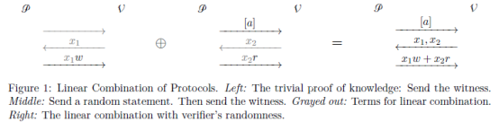

以上协议具有可extractable特性，当针对相同的 r ⃗ \vec{r} r ，Verifier给两组不同的challenges x ⃗ 1 , x ⃗ 2 \vec{x}_1,\vec{x}_2 x 1​,x 2​，Prover返回两组不同的response z ⃗ 1 , z ⃗ 2 \vec{z}_1,\vec{z}_2 z 1​,z 2​，从而可extract提取出witness w ⃗ \vec{w} w 和 randomness r ⃗ \vec{r} r 。 同理，这种类型的linear combination也可用于恢复batch proofs（参见Peng等人2007年论文《Batch zero-knowledge proof and verification and its applications》），non-randomised linear combinations也适合（参见Bünz 等人2018年论文《Bulletproofs: Short Proofs for Confidential Transactions and More》）。

1.2.3 Uniform(-or-unique) response

是指Prover反馈的response只有两种可能：

• uniformly distributed (conditioned on all later messages, not previous messages)，如1.2节中的 z ⃗ \vec{z} z 。
• 可以uniquely determined and efficiently computable from the challenges and all later messages，如1.2节中的 [ a ] [\mathbf{a}] [a]。

对Prover response的这个要求，有利于构建trivial simulator——反向运行transcript：从最终的消息开始，依次反推至最初的消息。这样simulator就可以自己选择uniformly distributed messages，然后计算出uniquely determined ones。

1.2.4 Kernels and redundancy

可参看博客 Ker(A)——矩阵kernel。

很多有趣的statement都是非线性的。 以 Bootle和Groth 2018年论文《Efficient Batch Zero-Knowledge Arguments for Low Degree Polynomials》中的polynomial commitment为例，a polynomial f ∈ F p [ X ] f\in\mathbb{F}_p[X] f∈Fp​[X]， f ( X ) = a 0 + a 1 X + ⋯ + a n − 1 X n − 1 f(X)=a_0+a_1X+\cdots+a_{n-1}X^{n-1} f(X)=a0​+a1​X+⋯+an−1​Xn−1，对于任意的 x ∈ F p x\in\mathbb{F}_p x∈Fp​，需证明 f ( x ) = t f(x)=t f(x)=t。 最直观的方法是：直接对 f ( X ) f(X) f(X)中所有的系数 a 0 , ⋯   , a n − 1 a_0,\cdots,a_{n-1} a0​,⋯,an−1​进行commit，然后借助linear combination protocol就可证明 f ( x ) = t f(x)=t f(x)=t成立。 但是，如果想实现random linear combination，可在不影响soundness的情况下增加redundancy，通过巧妙地对 ”evaluate at x x x”-map 创建 a non-trivial kenerl，具体实现方式为：将 f ( X ) f(X) f(X)表示为 f ( X ) = ∑ i ( α i + β i ) X i f(X)=\sum_{i}(\alpha_i+\beta_i)X^i f(X)=∑i​(αi​+βi​)Xi，然后对所有的 α i \alpha_i αi​和 β i \beta_i βi​进行commit。同理，若想表示 f ( x ) = 0 f(x)=0 f(x)=0，可直接取 α i ← F p , β i = − α i \alpha_i\leftarrow\mathbb{F}_p,\beta_i=-\alpha_i αi​←Fp​,βi​=−αi​。 从而在response中插入了randomness，总之可通过增加redundancy的方式来实现uniformly random responses。

1.2.5 argument systems组合

以inner product argument I P A a l m Z K IPA_{almZK} IPAalmZK​为例，需证明： ∃ x ⃗ , y ⃗ : < x ⃗ , y ⃗ > = t \exists \vec{x},\vec{y}:=t ∃x ,y ​:=t 引入随机数，转为证明：（仅需要logarithmically many (specially chosen) random components in r ⃗ , s ⃗ \vec{r},\vec{s} r ,s 。） < x ⃗ + r ⃗ , y ⃗ + s ⃗ > = t =t =t，其中 < r ⃗ , y ⃗ > = < r ⃗ , s ⃗ > = < x ⃗ , s ⃗ > = 0 ===0 ===0

这就是“redundancy/kernel”技术的一种应用。而“uniform-or-unique”指南可保证每次response都是随机的。从而在 r ⃗ , s ⃗ \vec{r},\vec{s} r ,s 中仅需要a logarithmic number of (well-chosen) random components 就足够了。

1.3 本文主要贡献 1.3.1 linear map preimage argument (LMPA)

分两步来实现对 ∃ w ⃗ : [ A ] w ⃗ = [ t ⃗ ] \exists\vec{w}:[\mathbf{A}]\vec{w}=[\vec{t}] ∃w :[A]w =[t ]（其中 [ A ] ∈ G m × n [\mathbf{A}]\in\mathbb{G}^{m\times n} [A]∈Gm×n） 的证明，具有的communication complexity为 O ( log ⁡ ( n ) ) O(\log(n)) O(log(n))：（参见1.2.1节内容。）

• 首先，使用batch verification L M P A b a t c h LMPA_{batch} LMPAbatch​，在方程式左侧乘以一个随机向量 y ⃗ ∈ F p m \vec{y}\in\mathbb{F}_p^m y ​∈Fpm​，获得 [ A ⃗ ^ ] = y ⃗ T [ A ] ∈ G 1 × n , [ t ^ ] = y ⃗ T [ t ] ∈ G [\hat{\vec{A}}]=\vec{y}^T[\mathbf{A}]\in\mathbb{G}^{1\times n},[\hat{t}]=\vec{y}^T[\mathbf{t}]\in\mathbb{G} [A ^]=y ​T[A]∈G1×n,[t^]=y ​T[t]∈G。此时，实现了communication cost与 m m m无关。
• 然后，使用 L M P A z k LMPA_{zk} LMPAzk​协议来证明 ∃ w ⃗ : [ A ⃗ ^ ] w ⃗ = [ t ^ ] \exists\vec{w}:[\hat{\vec{A}}]\vec{w}=[\hat{t}] ∃w :[A ^]w =[t^]。其中 L M P A z k LMPA_{zk} LMPAzk​协议源自Bootle等人2016年论文《Efficient Zero-Knowledge Arguments for Arithmetic Circuits in the Discrete Log Setting》中算法，并在此基础上实现了zero-knowledge，代价是增加了constant communication overhead和logarithmic computational overhead (in n n n)。

1.3.2 quadratic equation commit-and-prove

在Bootle等人2016年论文《Efficient Zero-Knowledge Arguments for Arithmetic Circuits in the Discrete Log Setting》和Bünz 等人2018年论文《Bulletproofs: Short Proofs for Confidential Transactions and More》的基础上，本文实现了一个 (almost) zero-knowledge inner product argument I P A a l m Z K IPA_{almZK} IPAalmZK​协议，代价是增加了constant communication overhead和logarithmic computational overhead。 I P A a l m Z K IPA_{almZK} IPAalmZK​协议用于证明的内容为 ∃ w ⃗ : ∀ i : < w ⃗ , Γ i w ⃗ > = 0 \exists\vec{w}:\forall i :=0 ∃w :∀i:=0，其中 Γ i ∈ F p n × n \mathbf{\Gamma_i}\in\mathbb{F}_p^{n\times n} Γi​∈Fpn×n​， w ⃗ \vec{w} w 为committed to。 为提升效率，采用batch proof方式，改为证明 < w ⃗ , Γ w ⃗ > ，其中 Γ = ∑ i r i Γ i \mathbf{\Gamma}=\sum_{i}r_i\Gamma_i Γ=∑i​ri​Γi​ for random r i ∈ F p r_i\in\mathbb{F}_p ri​∈Fp​。 最终生成的argument可称为 Q E S A Z K QESA_{ZK} QESAZK​，具有”adaptive commit-and-prove”特性，即the statement Γ i \mathbf{\Gamma_i} Γi​ may be chosen after the commitment to w ⃗ \vec{w} w 。

commit-and-prove system Q E S A Z K QESA_{ZK} QESAZK​ 理论简单且可与其它arguments高效结合使用。

1.3.3 quadratic equations集合

不借助R1CS，证明任意的quadratic equations如 ( ∑ a i x i ) ( ∑ b i x i ) + ∑ c i x i = 0 (\sum a_ix_i)(\sum b_ix_i)+\sum c_ix_i=0 (∑ai​xi​)(∑bi​xi​)+∑ci​xi​=0。 可将quadratic equation表示为 < x ⃗ , x ⃗ > = ∑ x i 2 = t =\sum x_i^2=t =∑xi2​=t，而若采用R1CS来表示，则需要 n n n个方程式： y i = x i 2 ( i = 1 , ⋯   , n − 1 ) y_i=x_i^2(i=1,\cdots,n-1) yi​=xi2​(i=1,⋯,n−1) and x n 2 = t − ∑ i y i x_n^2=t-\sum_{i}y_i xn2​=t−∑i​yi​，其中 y i y_i yi​为额外引入的变量。

Q E S A Z K QESA_{ZK} QESAZK​ 仅需要一个（quadratic）equation来表示 < x ⃗ , x ⃗ > = t =t =t。

借助这种表示，可对任意degree为 d 2 − 1 d^2-1 d2−1 的（univariate）多项式 f ( X ) = ∑ i = 1 d 2 − 1 a i X i f(X)=\sum_{i=1}^{d^2-1}a_iX^i f(X)=∑i=1d2−1​ai​Xi 以 2 d 2d 2d 个equations和intermediate variables来表示： y i = x i = y i − 1 x y_i=x^i=y_{i-1}x yi​=xi=yi−1​x 其中 i = 1 , ⋯   , d ， y 0 = 1 i=1,\cdots,d，y_0=1 i=1,⋯,d，y0​=1 z i = x d i = z 1 z i − 1 z_i=x^{di}=z_1z_{i-1} zi​=xdi=z1​zi−1​ 其中 i = 2 , ⋯   , d − 1 ， z 1 = y d − 1 x ， z 0 = 1 i=2,\cdots,d-1，z_1=y_{d-1}x，z_0=1 i=2,⋯,d−1，z1​=yd−1​x，z0​=1 最终 f ( x ) = ∑ i , j = 0 d , d − 1 a i + j d y i z j f(x)=\sum_{i,j=0}^{d,d-1}a_{i+jd}y_iz_j f(x)=∑i,j=0d,d−1​ai+jd​yi​zj​。

对于S(N)ARK-friendly cryptography （Kosba等人2015年论文《“C∅C∅: A Framework for Building Composable Zero-Knowledge Proof》），支持quadratic equations 将非常有用。Matrix-vector multiplications将可快速计算，即使matrix和vector 二者都是secret的。采用类似 Jubjub 的embedding elliptic curve，其效率要优于R1CS。对于general point addition in a (twisted) Edwards curve，不再需要8个，仅需要5个constraints per bit就足够了。

1.3.4 实现shuffle证明

采用本文的 L M P A Z K LMPA_{ZK} LMPAZK​和 Q E S A Z K QESA_{ZK} QESAZK​协议可实现 Stephanie Bayer和Jens Groth 2012年论文《Efficient Zero-Knowledge Argument for Correctness of a Shuffle》中的shuffle证明算法。 （参见博客 Efficient Zero-Knowledge Argument for Correctness of a Shuffle学习笔记（1））

本文构建的shuffle证明算法 Π s h u f f l e \Pi_{shuffle} Πshuffle​ 可证明 correctness of a shuffle (of EIGamal ciphertexts)，具有的proof size为 O ( log ⁡ ( N ) ) O(\log(N)) O(log(N))，而Stephanie Bayer和Jens Groth 2012年论文的proof size为 O ( N ) O(\sqrt{N}) O(N ​)。

1.3.5 short-circuit extraction

2. 相关安全假设

Instead of discrete logarithm assumptions, Morillo等人2016年论文《The Kernel Matrix Diffie-Hellman Assumption》中提及的the generalization of hard (matrix) kernel assumptions, but for right-kernels, better suits our needs。

• hard kernel assumption：（与Pedersen commitment的binding属性关联。Breaking the binding property of the commitment is equivalent to finding non-trivial elements in k e r ( [ A ] ) ker([\mathbf{A}]) ker([A])。）

3. Matrix-vector multiplication argument

c k = [ g ⃗ ] = [ g 0 , g ˉ ⃗ ] ← G 1 + 1 × n ck=[\vec{g}]=[g_0,\vec{\bar{g}}]\leftarrow \mathbb{G}^{1+1\times n} ck=[g ​]=[g0​,gˉ​ ​]←G1+1×n 为Pedersen commitment key。其中 g 0 ∈ G , [ g ˉ ⃗ ] ∈ G n g_0\in\mathbb{G},[\vec{\bar{g}}]\in\mathbb{G}^n g0​∈G,[gˉ​ ​]∈Gn。 定义 C o m g ( w ⃗ ; r ) = [ g 0 ] r + [ g ˉ ⃗ ] w ⃗ Com_{g}(\vec{w};r)=[g_0]r+[\vec{\bar{g}}]\vec{w} Comg​(w ;r)=[g0​]r+[gˉ​ ​]w for r ∈ F p , w ⃗ ∈ F p n r\in\mathbb{F}_p,\vec{w}\in\mathbb{F}_p^n r∈Fp​,w ∈Fpn​ 矩阵 [ A ] ∈ G m × n [\mathbf{A}]\in\mathbb{G}^{m\times n} [A]∈Gm×n 向量 w ⃗ ∈ F p n , [ t ⃗ ] ∈ G m \vec{w}\in\mathbb{F}_p^n, [\vec{t}]\in\mathbb{G}^m w ∈Fpn​,[t ]∈Gm

为了证明 ∃ w ⃗ : [ A ] w ⃗ = [ t ⃗ ] \exists\vec{w}:[\mathbf{A}]\vec{w}=[\vec{t}] ∃w :[A]w =[t ]，本文主要遵循2个原则：

• 使用 probabilistic (batch) verification来check many things at once；
• 若messages are too long, replace them by a shorter proof (of knowledge)。（采用shrinking commitments来keep the messages small。）

基本信息为：

• Public info： [ A ] ∈ G m × n [\mathbf{A}]\in\mathbb{G}^{m\times n} [A]∈Gm×n， [ t ⃗ ] ∈ G m [\vec{t}]\in\mathbb{G}^m [t ]∈Gm
• Private info： w ⃗ ∈ F p n \vec{w}\in\mathbb{F}_p^n w ∈Fpn​
• Relation： [ A ] w ⃗ = [ t ⃗ ] [\mathbf{A}]\vec{w}=[\vec{t}] [A]w =[t ]

Matrix-vector multiplication argument具有可组合性：

3.1 采用标准的 ∑ \sum ∑-protocol来证明Matrix-vector multiplication argument

若采用 Cramer等人1998年论文《Zero-Knowledge Proofs for Finite Field Arithmetic; or: Can Zero-Knowledge Be for Free?》和Maurer 2015年论文《Zero-knowledge proofs of knowledge for group homomorphisms》 中标准的 ∑ \sum ∑-protocol 来证明Matrix-vector multiplication argument，详细的实现思路为：（ ∑ s t d \sum_{std} ∑std​协议）

• Prover：选择随机向量 r ⃗ ← F p n \vec{r}\leftarrow\mathbb{F}_p^n r ←Fpn​，计算 [ a ⃗ ] = [ A ] r ⃗ [\vec{a}]=[\mathbf{A}]\vec{r} [a ]=[A]r ，将 [ a ⃗ ] ∈ G m [\vec{a}]\in\mathbb{G}^m [a ]∈Gm发送给Verifier。
• Verifier：选择随机数 β ← F p \beta\leftarrow\mathbb{F}_p β←Fp​。
• Prover：计算 z ⃗ = β w ⃗ + r ⃗ \vec{z}=\beta\vec{w}+\vec{r} z =βw +r ，将 z ⃗ ∈ F p n \vec{z}\in\mathbb{F}_p^n z ∈Fpn​发送给Verifier。
• Verifier：验证 [ A ] z ⃗ = β [ t ⃗ ] + [ a ⃗ ] [\mathbf{A}]\vec{z}=\beta[\vec{t}]+[\vec{a}] [A]z =β[t ]+[a ]是否成立即可。

以上基于标准 ∑ \sum ∑-protocol的整个实现communication cost为 O ( m + n ) O(m+n) O(m+n)。需要从以下两方面进行改进：

• 借助batch verification，使得communication与 m m m无关；（此处 m m m 为 number of equations。）
• 借助 Bootle等人2016年论文《Efficient Zero-Knowledge Arguments for Arithmetic Circuits in the Discrete Log Setting》和 Bünz 等人2018年论文《Bulletproofs: Short Proofs for Confidential Transactions and More》 中的递归方法，使得communication cost 为 O ( log ⁡ ( n ) ) O(\log(n)) O(log(n))。（此处 n n n 为witness size。）

3.2 借助batch verification 使communication与 m m m无关

需要shrink 3.1节中的 [ a ⃗ ] ∈ G m [\vec{a}]\in\mathbb{G}^m [a ]∈Gm，方法是将 m m m 个linear equations batch into a single linear equation。 详细的实现思路如下：（ L M P A b a t c h LMPA_{batch} LMPAbatch​协议）

• Prover：选择blind 随机数 r w ← F p r_w\leftarrow \mathbb{F}_p rw​←Fp​，计算 [ c w ] = [ g 0 ] r w + [ g ˉ ⃗ ] w ⃗ = C o m ( w ⃗ ; r w ) [c_w]=[g_0]r_w+[\vec{\bar{g}}]\vec{w}=Com(\vec{w};r_w) [cw​]=[g0​]rw​+[gˉ​ ​]w =Com(w ;rw​)。将 [ c w ] [c_w] [cw​]发送给Verifier。（即先对witness进行commit。）
• Verifier：选择随机数 x ← F p x\leftarrow \mathbb{F}_p x←Fp​，构建随机向量 x ⃗ = ( 1 , x , ⋯   , x m − 1 ) \vec{x}=(1,x,\cdots,x^{m-1}) x =(1,x,⋯,xm−1)，将 x ⃗ \vec{x} x 发送给Prover。
• Prover和Verifier：都计算 [ A ⃗ ^ ] = x ⃗ T [ A ] ∈ G 1 × n ， [ t ^ ] = x ⃗ T [ t ⃗ ] ∈ G [\hat{\vec{A}}]=\vec{x}^T[\mathbf{A}]\in\mathbb{G}^{1\times n}，[\hat{t}]=\vec{x}^T[\vec{t}]\in\mathbb{G} [A ^]=x T[A]∈G1×n，[t^]=x T[t ]∈G。具有 [ B ] = [ g 0 g ˉ ⃗ 0 A ⃗ ^ ] [\mathbf{B}]= \begin{bmatrix} g_0 & \vec{\bar{g}}\\ 0 & \hat{\vec{A}} \end{bmatrix} [B]=[g0​0​gˉ​ ​A ^​]，转为证明 ∃ : [ B ] ( r w w ⃗ ) = [ c w t ^ ] = [ u ⃗ ] \exists: [\mathbf{B}] \begin{pmatrix} r_w\\ \vec{w} \end{pmatrix} =\begin{bmatrix} c_w\\ \hat{t} \end{bmatrix}=[\vec{u}] ∃:[B](rw​w ​)=[cw​t^​]=[u ]，其中 [ B ] , [ u ⃗ ] [\mathbf{B}],[\vec{u}] [B],[u ] 为public info。从而可以继续采用3.1节的 ∑ \sum ∑-protocol来证明，调用 ∑ s t d \sum_{std} ∑std​子协议即可。

整个 L M P A b a t c h LMPA_{batch} LMPAbatch​协议为 5 5 5-move HVZK-AoK。

3.3 借助递归调用来 batch the witness

借助 Bootle等人2016年论文《Efficient Zero-Knowledge Arguments for Arithmetic Circuits in the Discrete Log Setting》和 Bünz 等人2018年论文《Bulletproofs: Short Proofs for Confidential Transactions and More》 中的递归方法，使得communication cost 为 O ( log ⁡ ( n ) ) O(\log(n)) O(log(n))。（此处 n n n 为witness size。）

首先构建相应的argument，然后再添加zero-knowledge。

在3.2节的基础上，可压缩为 m = 1 m=1 m=1。

k ∈ N , k ∣ n k\in\mathbb{N},k|n k∈N,k∣n，即 n / k ∈ N n/k\in\mathbb{N} n/k∈N。 将 [ A ] w ⃗ = [ t ⃗ ] [\mathbf{A}]\vec{w}=[\vec{t}] [A]w =[t ] reduce为 [ A ^ ] w ⃗ ^ = [ t ⃗ ^ ] [\hat{\mathbf{A}}]\hat{\vec{w}}=[\hat{\vec{t}}] [A^]w ^=[t ^]，其中 [ A ^ ] ∈ G m × n / k , w ⃗ ^ ∈ F p n / k , [ t ⃗ ^ ] ∈ G m [\hat{\mathbf{A}}]\in\mathbb{G}^{m\times n/k}, \hat{\vec{w}}\in\mathbb{F}_p^{n/k},[\hat{\vec{t}}]\in\mathbb{G}^m [A^]∈Gm×n/k,w ^∈Fpn/k​,[t ^]∈Gm。 将 [ A ] [\mathbf{A}] [A]和 w ⃗ \vec{w} w 切分为 k k k个equal blocks，有： [ A ] = [ A 1 ∣ ⋯ ∣ A k ] ∈ ( G m × n / k ) 1 × k [\mathbf{A}]=[\mathbf{A}_1|\cdots|\mathbf{A}_k]\in(\mathbb{G}^{m\times n/k})^{1\times k} [A]=[A1​∣⋯∣Ak​]∈(Gm×n/k)1×k，其中 [ A i ] ∈ G m × n / k [\mathbf{A}_i]\in\mathbb{G}^{m\times n/k} [Ai​]∈Gm×n/k，同理 w ⃗ = ( w 1 ⋯ w k ) ∈ ( G n / k ) k \vec{w}=\begin{pmatrix} w_1\\ \cdots \\ w_k \end{pmatrix}\in(\mathbb{G}^{n/k})^k w =⎝⎛​w1​⋯wk​​⎠⎞​∈(Gn/k)k。 转换为需证明： ∑ i = 1 k [ A i ] w ⃗ i = [ t ⃗ ] \sum_{i=1}^{k}[\mathbf{A}_i]\vec{w}_i=[\vec{t}] ∑i=1k​[Ai​]w i​=[t ]

采用Bootle等人2016年论文《Efficient Zero-Knowledge Arguments for Arithmetic Circuits in the Discrete Log Setting》中的思路，直接将其展开为：

其中右侧矩阵中主对角线上所有元素即为待证明的内容 ∑ i = 1 k [ A i ] w i ⃗ = [ t ⃗ ] \sum_{i=1}^{k}[\mathbf{A}_i]\vec{w_i}=[\vec{t}] ∑i=1k​[Ai​]wi​ ​=[t ] 有两种证明思路：

• 方法一： – Prover：将矩阵中的所有元素 [ A i ] w ⃗ j [\mathbf{A}_i]\vec{w}_j [Ai​]w j​发送给Verifier； – Verifier：为矩阵左侧构建challenge vector x ⃗ ∈ F p k = ( 1 , x , ⋯   , x k − 1 ) \vec{x}\in\mathbb{F}_p^k=(1,x,\cdots,x^{k-1}) x ∈Fpk​=(1,x,⋯,xk−1)，为矩阵右侧构建challenge vector y ⃗ ∈ F p k = ( 1 , y , ⋯   , y k − 1 ) \vec{y}\in\mathbb{F}_p^k=(1,y,\cdots,y^{k-1}) y ​∈Fpk​=(1,y,⋯,yk−1)。将 x ⃗ , y ⃗ \vec{x},\vec{y} x ,y ​ 发送给Prover； – Prover：利用矩阵运算结合律有：

此时Prover可发送 [ u ⃗ i , j ] = [ A i ] w ⃗ j [\vec{u}_{i,j}]=[\mathbf{A}_i]\vec{w}_j [u i,j​]=[Ai​]w j​，以及shrunk witness w ⃗ ^ \hat{\vec{w}} w ^。【注意此时不具有zero-knowledge。】 – Verifier：验证 ∑ i [ u ⃗ i , i ] = [ t ⃗ ] \sum_{i}[\vec{u}_{i,i}]=[\vec{t}] ∑i​[u i,i​]=[t ]和 [ A ^ ] w ⃗ ^ = [ h a t t ⃗ ] = ∑ i , j x i y j [ u ⃗ i , j ] [\hat{\mathbf{A}}]\hat{\vec{w}}=[hat{\vec{t}}]=\sum_{i,j}x_iy_j[\vec{u}_{i,j}] [A^]w ^=[hatt ]=∑i,j​xi​yj​[u i,j​]是否成立？ 若每个 [ A i ] [\mathbf{A}_i] [Ai​]都满足hard kernel assumption，则the prover is committed to w ⃗ 1 , ⋯   , w ⃗ k \vec{w}_1,\cdots,\vec{w}_k w 1​,⋯,w k​。不难发现若有足够多的challenges，则可extract w ⃗ \vec{w} w （or find non-trivial kernel elements）。以上方法，可将statement ( [ A ] , [ t ⃗ ] ) ([\mathbf{A}],[\vec{t}]) ([A],[t ]) reduce 为 ( [ A ^ ] , [ t ⃗ ^ ] ) ([\hat{\mathbf{A}}],[\hat{\vec{t}}]) ([A^],[t ^])，减小了 k k k倍。可递归调用再次reduce。

• 方法二：（借助了Bootle 2016论文中的思路） – Prover：与方法一不同，Prover不再发送矩阵中的所有元素，而只让Verifier知道各个对角线元素之和 [ u ⃗ l ] = ∑ j − i = l [ A i ] w ⃗ j [\vec{u}_l]=\sum_{j-i=l}[\mathbf{A}_i]\vec{w}_j [u l​]=∑j−i=l​[Ai​]w j​，其中 l = ± 1 , ⋯   , ± k l=\pm 1,\cdots,\pm k l=±1,⋯,±k，且 [ u ⃗ 0 ] = [ t ⃗ ] [\vec{u}_0]=[\vec{t}] [u 0​]=[t ]。 – Verifier：为了让 ∑ i , j x i y j [ A i ] w ⃗ j = z l ∑ j − i = l [ A i ] w ⃗ j \sum_{i,j}x_iy_j[\mathbf{A}_i]\vec{w}_j=z_l\sum_{j-i=l}[\mathbf{A}_i]\vec{w}_j ∑i,j​xi​yj​[Ai​]w j​=zl​∑j−i=l​[Ai​]w j​，则相应的 challenge vectors需调整为 x ⃗ ∈ F p k = ( 1 , x , ⋯   , x k − 1 ) \vec{x}\in\mathbb{F}_p^k=(1,x,\cdots,x^{k-1}) x ∈Fpk​=(1,x,⋯,xk−1)， y ⃗ ∈ F p k = ( 1 , x − 1 , ⋯   , x − k + 1 ) \vec{y}\in\mathbb{F}_p^k=(1,x^{-1},\cdots,x^{-k+1}) y ​∈Fpk​=(1,x−1,⋯,x−k+1)，此时 z l = x − l z_l=x^{-l} zl​=x−l【或者更高效的方式是，构建 y ⃗ ∈ F p k = ( x k − 1 , x k − 2 , ⋯   , x , 1 ) \vec{y}\in\mathbb{F}_p^k=(x^{k-1},x^{k-2},\cdots,x,1) y ​∈Fpk​=(xk−1,xk−2,⋯,x,1)，此时 z l = x k − 1 − l z_l=x^{k-1-l} zl​=xk−1−l】。将 x ⃗ , y ⃗ \vec{x},\vec{y} x ,y ​ 发送给Prover； 详细的 L M P A n o Z K LMPA_{noZK} LMPAnoZK​协议为：

L M P A n o Z K LMPA_{noZK} LMPAnoZK​协议具有recursive extraction特性：

4. Matrix-vector multiplication argument + Zero-Knowledge

3.2节和3.3节的Matrix-vector multiplication argument均不具有zero-knowledge，而3.1节中的communication cost为 O ( m + n ) O(m+n) O(m+n)，为实现Matrix-vector multiplication argument + Zero-Knowledge 的基本思路有：

• 方法一： ∑ s t d \sum_{std} ∑std​协议+ L M P A n o Z K LMPA_{noZK} LMPAnoZK​协议= L M P A s i m p l e Z K LMPA_{simpleZK} LMPAsimpleZK​协议 借助3.1节中的 ∑ s t d \sum_{std} ∑std​协议，不再直接发送 z ⃗ ∈ F p n \vec{z}\in\mathbb{F}_p^n z ∈Fpn​使得 ∃ z ⃗ : [ A ] z ⃗ = β [ t ⃗ ] + [ a ⃗ ] \exists \vec{z}:[\mathbf{A}]\vec{z}=\beta[\vec{t}]+[\vec{a}] ∃z :[A]z =β[t ]+[a ]，而转为调用 L M P A n o Z K LMPA_{noZK} LMPAnoZK​协议来证明。 L M P A s i m p l e Z K LMPA_{simpleZK} LMPAsimpleZK​协议具有communication efficiency，但是对于random r ⃗ \vec{r} r ，计算 [ A ] r ⃗ [\mathbf{A}]\vec{r} [A]r 是expensive的。与Bootle 2016和Bünz 2018方案类似， L M P A n o Z K LMPA_{noZK} LMPAnoZK​协议仅用于save communication。

• 方法二： 方法一是对所有的witness进行了blinding，实际是仅对Prover’s response进行blind就足够了，这样 a logarithmic amount of randomness 就足够了，从而可以提高Prover的计算效率。

4.1 zero knowledge of opening of a commitment.

假设 [ A ] = [ g ⃗ ] ∈ G 1 × n [\mathbf{A}]=[\vec{g}]\in\mathbb{G}^{1\times n} [A]=[g ​]∈G1×n，其中 [ g ⃗ ] [\vec{g}] [g ​]为commitment key， k = 2 k=2 k=2。 [ A ] [\mathbf{A}] [A]满足hard kernel assumption by construction。 转为构建zero-knowledge argument for ∃ w ⃗ : [ g ⃗ ] w ⃗ = [ t ] \exists\vec{w}:[\vec{g}]\vec{w}=[t] ∃w :[g ​]w =[t]。 与 ∑ s t d \sum_{std} ∑std​协议中的实现不同，通过明智地选择randomness r ⃗ \vec{r} r 来构建masked version of L M P A n o Z K LMPA_{noZK} LMPAnoZK​。不再是随机选择 r ⃗ ← F p n \vec{r}\leftarrow\mathbb{F}_p^n r ←Fpn​，而是只选择logarithmically个非零的 r i r_i ri​值，其它的均为零值，从而使得计算 [ g ⃗ ] r ⃗ = [ a ] [\vec{g}]\vec{r}=[a] [g ​]r =[a]非常cheap。

从而借助Masking sets来构建challenge r ⃗ ← M n \vec{r}\leftarrow \mathbb{M}_n r ←Mn​，可实现计算压力更小的zero-knowledge argument：

4.2 zero knowledge of Matrix-vector multiplication argument

对于更general的 [ A ] ∈ G m × n [\mathbf{A}]\in\mathbb{G}^{m\times n} [A]∈Gm×n，相对于4.1节，难点主要在：

• 对 m > 1 m>1 m>1的情况构建masking sets不再直观可实现，由于 u ⃗ l ∈ G m \vec{u}_l\in\mathbb{G}^m u l​∈Gm，Prover需要communicate m k mk mk elements，从而需要 m k log ⁡ ( n ) mk\log(n) mklog(n)个random entries来randomise all of [ u ⃗ l ] [\vec{u}_l] [u l​]。而直观的 ∑ s t d \sum_{std} ∑std​协议仅需要 n n n个random entries。
• making the definition of M n \mathbb{M}_n Mn​ dynamic and depend on [ A ] [\mathbf{A}] [A] is inconvenient and hard。需借助commitment-extension方法，如Bootle 2016方案中是通过引入随机数行来实现computationally injective，而本文是通过引入随机数列来实现surjective。由证明 [ t ⃗ ] = [ A ] w ⃗ [\vec{t}]=[\mathbf{A}]\vec{w} [t ]=[A]w 改为证明 [ B ⃗ ] = [ A ∣ H ] ( w ⃗ r ⃗ ) [\vec{B}]=[\mathbf{A}|\mathbf{H}]\begin{pmatrix} \vec{w}\\ \vec{r} \end{pmatrix} [B ]=[A∣H](w r ​)。

详细的 L M P A a l m S n d LMPA_{almSnd} LMPAalmSnd​实现为：

对以上协议中的matrix [ h ] [\mathbf{h}] [h] 进一步优化，使其基于common reference string来生成，not adversarial，最终的 L M P A Z K LMPA_{ZK} LMPAZK​协议为：

5. 基于quadratic equations来构建arithmetic circuit satisfiability 5.1 quadratic gate表示

本文针对的场景为：（commit-and-prove system）

• witness： w ⃗ ∈ F p n \vec{w}\in\mathbb{F}_p^n w ∈Fpn​；
• public info：matrix Γ ∈ F p n × n \mathbf{\Gamma}\in\mathbb{F}_p^{n\times n} Γ∈Fpn×n​；
• relation： w ⃗ T Γ w ⃗ = 0 \vec{w}^T\mathbf{\Gamma}\vec{w}=0 w TΓw =0

与Groth等人2008年论文《Efficient Non-interactive Proof Systems for Bilinear Groups》 和 Escala等人2014年论文《Fine-Tuning Groth-Sahai Proofs》中的定义类似，约定 w 1 = 1 w_1=1 w1​=1。

对于更general的quadratic equation x ⃗ T Γ x ⃗ + a ⃗ T x ⃗ = t \vec{x}^T\mathbf{\Gamma}\vec{x}+\vec{a}^T\vec{x}=t x TΓx +a Tx =t，其中 a ⃗ , x ⃗ ∈ F p n , Γ ∈ F p n × n , t ∈ F p \vec{a},\vec{x}\in\mathbb{F}_p^n,\mathbf{\Gamma}\in\mathbb{F}_p^{n\times n},t\in\mathbb{F}_p a ,x ∈Fpn​,Γ∈Fpn×n​,t∈Fp​，public info为KaTeX parse error: Expected 'EOF', got '}' at position 25: …\mathbf{\Gamma}}̲,t)，也可转换为如上quadratic gate表示： 设置 w ⃗ = ( 1 x ⃗ ) \vec{w}=\begin{pmatrix} 1\\ \vec{x} \end{pmatrix} w =(1x ​)，从而有 w ⃗ T ( − t 0 a ⃗ Γ ) w ⃗ = 0 \vec{w}^T\begin{pmatrix} -t & 0\\ \vec{a} & \mathbf{\Gamma} \end{pmatrix}\vec{w}=0 w T(−ta ​0Γ​)w =0。

5.2 R1CS转quadratic equation

参见博客 rank-1 constraint system R1CS

R1CS的表示为： ( w ⃗ T a ⃗ ) ( b ⃗ T w ⃗ ) − c ⃗ T w ⃗ = 0 (\vec{w}^T\vec{a})(\vec{b}^T\vec{w})-\vec{c}^T\vec{w}=0 (w Ta )(b Tw )−c Tw =0，其中 a ⃗ , b ⃗ , c ⃗ ∈ F p n \vec{a},\vec{b},\vec{c}\in\mathbb{F}_p^n a ,b ,c ∈Fpn​ 设置 Γ = a ⃗ b ⃗ T − e ⃗ 1 c ⃗ T \mathbf{\Gamma}=\vec{a}\vec{b}^T-\vec{e}_1\vec{c}^T Γ=a b T−e 1​c T，其中 e ⃗ 1 = ( 1 , 0 , 0 , ⋯   , 0 ) \vec{e}_1=(1,0,0,\cdots,0) e 1​=(1,0,0,⋯,0) 可将上述R1CS表示转为quadratic equation表示： w ⃗ T Γ w ⃗ = 0 \vec{w}^T\mathbf{\Gamma}\vec{w}=0 w TΓw =0

5.3 quadratic equation to inner product argument

由待证明的relation w ⃗ T Γ w ⃗ = 0 \vec{w}^T\mathbf{\Gamma}\vec{w}=0 w TΓw =0 观察可知，可看作 w ⃗ T Γ w ⃗ = < w ⃗ , Γ w ⃗ > \vec{w}^T\mathbf{\Gamma}\vec{w}= w TΓw =为an inner product，从而接下来的任务转为需要构建zero-knowledge inner-product argument。 若已知 Γ \mathbf{\Gamma} Γ，目前技术无法generate a commitment to Γ w ⃗ \mathbf{\Gamma}\vec{w} Γw efficiently。

• Prover：首先commit to w ⃗ \vec{w} w 为 [ c x ] = C o m c k 1 ( w ⃗ ) [c_x]=Com_{ck_1}(\vec{w}) [cx​]=Comck1​​(w )，然后根据 Γ \mathbf{\Gamma} Γ commit to Γ w ⃗ \mathbf{\Gamma}\vec{w} Γw 为 [ c y ] = C o m c k 2 ( G a m m a w ⃗ ) [c_y]=Com_{ck_2}(\mathbf{Gamma}\vec{w}) [cy​]=Comck2​​(Gammaw )。最后Prover执行the inner product argument。 Prover必须证明 [ c x ] [c_x] [cx​] open to x ⃗ = w ⃗ \vec{x}=\vec{w} x =w and [ c y ] [c_y] [cy​] open to y ⃗ = Γ x ⃗ \vec{y}=\mathbf{\Gamma}\vec{x} y ​=Γx 。 采用（linear）batching技术可进一步转为证明 y ⃗ = Γ x ⃗ \vec{y}=\mathbf{\Gamma}\vec{x} y ​=Γx ，为了验证 y ⃗ = Γ x ⃗ \vec{y}=\mathbf{\Gamma}\vec{x} y ​=Γx 成立，Verifier可提供challenge s ⃗ ← F p n \vec{s}\leftarrow\mathbb{F}_p^n s ←Fpn​，Prover证明 0 = < Γ x ⃗ − y ⃗ , s ⃗ > 0= 0=。

从而为了证明 w ⃗ T Γ w ⃗ = 0 \vec{w}^T\mathbf{\Gamma}\vec{w}=0 w TΓw =0，可拆分为两个子inner product 证明：（其中 x ⃗ = w ⃗ , y ⃗ = Γ w ⃗ \vec{x}=\vec{w},\vec{y}=\mathbf{\Gamma}\vec{w} x =w ,y ​=Γw ）

• < x ⃗ , y ⃗ > = 0 =0 =0
• < Γ x ⃗ − y ⃗ , s ⃗ > = 0 =0 =0

可将以上两个inner product 证明batch为一个inner product，由Verifier提供challenge α \alpha α，构建witness 为 x ⃗ , y ⃗ \vec{x},\vec{y} x ,y ​的待证明relation为：

接下来的重点是构建zero-knowledge inner product argument。

5.4 zero-knowledge inner product argument

Bootle 2016和Bünz 2018方案中的inner product argument不具有zero-knowledge。 I P A n o Z K IPA_{noZK} IPAnoZK​将Bootle 2016和Bünz 2018方案进行了整合：

有多种方式来为inner product argument添加zero-knowledge属性：

• L M P A Z K LMPA_{ZK} LMPAZK​是通过采用linear combination (with “extended randomness”) 来attain zero-knowledge。
• 直接对witness进行mask，如构建 < w ⃗ ’ + r ⃗ ’ , w ⃗ ’ ’ + r ⃗ ‘ ’ > ，由于具有非线性特性，仅给Verifier发送 t r = < r ⃗ ’ , r ⃗ ’ ’ > t_r= tr​=是不够的。若再发送 < w ⃗ ’ , r ⃗ ’ ’ > 和 < w ⃗ ’ ’ , r ⃗ ’ > 则不符合zero-knowledge要求。 若选择随机数 r ⃗ ’ , r ⃗ ’ ’ \vec{r}’,\vec{r}’’ r ’,r ’’采用 kernel guidline来选取：

I P A a l m Z K IPA_{almZK} IPAalmZK​协议的详细实现为：

5.5 quadratic equation satisfiability

对一系列的quadratic equations进行证明， Q E S A Z K QESA_{ZK} QESAZK​协议为：

5.6 combine Q E S A Z K QESA_{ZK} QESAZK​ with other proof systems

如基于 Q E S A C o p y QESA_{Copy} QESACopy​协议构建的range proof与Bulletproofs中构建的range proofs对比为：

6. 引申至add arithmetic circuit relations to the witness

若 [ A ] [\mathbf{A}] [A]的第一行为Pedersen commitment key [ g ⃗ ] [\vec{g}] [g ​]，则很容易 make other (zero-knowledge) statements about w ⃗ \vec{w} w by composition of zero-knowledge protocols。 如用于shuffle证明。

Stephanie Bayer和Jens Groth 2012年论文《Efficient Zero-Knowledge Argument for Correctness of a Shuffle》的shuffle argument 主要由两部分组成：（参见博客 Efficient Zero-Knowledge Argument for Correctness of a Shuffle学习笔记（1））

• a product argument；
• a multi-exponentiation argument。

本文基于 Q E S A Z K QESA_{ZK} QESAZK​或 Q E S A C o p y QESA_{Copy} QESACopy​构建的shuffle argument思路为：

Stephanie Bayer和Jens Groth 2012 的 shuffle argument proof size 为 O ( N ) O(\sqrt{N}) O(N ​)，而基于本文构建的 Q E S A Z K QESA_{ZK} QESAZK​的shuffle argument proof size为 O ( log ⁡ ( N ) ) O(\log(N)) O(log(N))。