以下链接是个人关于MVSNet(R-MVSNet)-多视角立体深度推导重建 所有见解,如有错误欢迎大家指出,我会第一时间纠正。有兴趣的朋友可以加微信:17575010159 相互讨论技术。若是帮助到了你什么,一定要记得点赞!因为这是对我最大的鼓励。 文末附带 \color{blue}{文末附带} 文末附带 公众号 − \color{blue}{公众号 -} 公众号− 海量资源。 \color{blue}{ 海量资源}。 海量资源。
3D点云重建0-00:MVSNet(R-MVSNet)–目录-史上最新无死角讲解:https://blog.csdn.net/weixin_43013761/article/details/102852209
代码引导改篇博客主要讲解的是Cost Volume Regularization以及soft_arg_min,但是Cost Volume Regularization没有什么好说的,其代码在mvsnet/train.py:
    # filtered cost volume, size of (B, D, H, W, 1)=(?, 192, ?, ?, 1)
    # 这里完成的是论文图示的Cost Volume Regularization操作,带有反卷积操作,对初始的cost_volume进行过滤
    if is_master_gpu:
        filtered_cost_volume_tower = RegNetUS0({'data': cost_volume}, is_training=True, reuse=False)
    else:
        filtered_cost_volume_tower = RegNetUS0({'data': cost_volume}, is_training=True, reuse=True)

    # 进行维度压缩得到[B, D, H, W]
    filtered_cost_volume = tf.squeeze(filtered_cost_volume_tower.get_output(), axis=-1)
对应论文图示:  可以理解为,就是使用3D卷积,对Cost Volume进行了过滤,或者说把视觉差信息,转化为能求深度图的信息。主要的要点在于,怎么能让网络去学习这个转化过程,下面我们来看看吧。从RegNetUS0的输入和输出,以及改部分网络是看出来的,我们需要往后琢磨代码。
这里我先把代码贴出来,当然还是在mvsnet/model.py里面:
    # depth map by softArgmin
    with tf.name_scope('soft_arg_min'):
        # probability volume by soft max
        # tf.scalar_mul为标量与矢量相乘,这里乘以-1,等于加上了-号,
        # 对3D立体的volume每个立体像素,都进行深度预测
        # probability_volume[B, D, H, W],
        # 这里的axis=1,也就是沿着D所在的轴,所有体素中存储的概率值相加为1
        probability_volume = tf.nn.softmax(
            tf.scalar_mul(-1, filtered_cost_volume), axis=1, name='prob_volume')


        # depth image by soft argmin
        # 获得probability_volume的形状[B, D, H, W]
        volume_shape = tf.shape(probability_volume)
        soft_2d = []
        # 对每个样本进行处理
        for i in range(FLAGS.batch_size):
            # 对每个样本,根据depth_start[i], depth_end[i]的不同,但是划分成depth_num份
            # tf.linspace使用,如tf.linspace(0,5,5)=[0,1,2,3,4]
            soft_1d = tf.linspace(depth_start[i], depth_end[i], tf.cast(depth_num, tf.int32))
            soft_2d.append(soft_1d)
        # [b,d,1,1]
        soft_2d = tf.reshape(tf.stack(soft_2d, axis=0), [volume_shape[0], volume_shape[1], 1, 1])
        # [b,d,h,w]
        soft_4d = tf.tile(soft_2d, [1, 1, volume_shape[2], volume_shape[3]])

        #estimated_depth_map[b,h,w], 这个地方注意以下,filtered_cost_volume是乘了-1之后再计算概率的,为的就是深度的反转
        # 把soft_4d现象成立体空间,因为前面是用tf.linspace生成,在D的方向存储的就是类似于1,2,3,4,5,6,7,..........这样的数据
        # 假设r img的一个像素,经过tf.nn.softmax进行预测,落在三维空间深度为5的地方,那么是不是除了5的概率接近1,其他地方的概率低接近0
        # (如果此时网络已经很好的收敛),5乘以一个接近1的数,他的值还是得5,其他的乘以一个接近0的数,那么结果接近为0
        # 下面在D的方向axis=1进行求和,他们的值还是5,对吧。就是一个5加了很多个0
        # 这样,我们就从二维空间先转到3维的概率空间,然后求和得到深度,有道理没?
        estimated_depth_map = tf.reduce_sum(soft_4d * probability_volume, axis=1)
        # [b,h,w,1]
        estimated_depth_map = tf.expand_dims(estimated_depth_map, axis=3)

    # 获得深度概率分布图
    prob_map = get_propability_map(probability_volume, estimated_depth_map, depth_start, depth_interval)
    return estimated_depth_map, prob_map#, filtered_depth_map, probability_volume
从上面我们可以看到,经过过滤得到的filtered_cost_volume,直接经过tf.nn.softmax进行分类处理,并且在这之前还乘以-1。得到的形状还是和filtered_cost_volume一样的,为[B, D, H, W]。注意的是tf.nn.softmax中的参数axis=1,表示的是按照深度来进行概率预算的。这个地方,比较就觉抽象,如下所示: 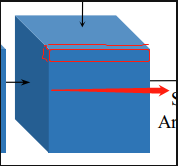 也就是上面红色部分(我已经尽力了),红色部分的体素中保存的概率值相加为1,可以看到根据长宽不一样,这个probability_volume可以分成很多个类似红框的部分。
这样预测出来的东西是什么,其表示的是2维图像映射到3维空间后,他应该在处于哪个深度,那么在probability_volume,这个深度对应的位置,其存储的概率值会最大,那么可以想到D方向(箭头方向)其他的体素存储的概率值都接近0。
还要理解的就是estimated_depth_map = tf.reduce_sum(soft_4d * probability_volume, axis=1),这个函数,其实就是计算的D方向的一个期望值。论文中的公式如下: D = ∑ d = d m i n d m a x d × P ( d ) D=\sum_{d=d_{min}}^{d_{max}}d \times P(d) D=d=dmin∑dmaxd×P(d)
到这里,我们已经知道了深度是怎么来的了,下面我们来看看概率图(Probability Map)。
Probability Map从上面我们可以找到:
	......
	# 获得深度概率分布图
    prob_map = get_propability_map(probability_volume, estimated_depth_map, depth_start, depth_interval)
	......
在讲解之前,我们来看看,概率的描述图:  c中上面的图示,表示的是非离群点(概率都集中在一个深度),下面的表示的是离群点(概率都比较分散)。造成利群点的原因是什么?因为他是背景,那么为什么背景就会出现利群点?在论文中,也有提到过,那就是背景是不会进行反向传播和优化的(具体细后面讲解)。背景因为比较离散,4个值,当做一个值,有点类似于平滑的效果,我们先看看代码吧:
def get_propability_map(cv, depth_map, depth_start, depth_interval):
    """
    get probability map from cost volume,
    该函数的主要作用,可以这样理解,一个(4,)的滑动窗口,在cv(probability_volume)
    滑动步伐为1,每滑动一次,都会把这四个像素存储的深度概率值都相加起来,
    当作一个概率图prob_map的一个像素,这样能够去除异常点的干扰。带着这个
    思路去分析,会比较简单

    cv: probability_volume[B, D, H, W],r img映射3维空间所处深度的概率值
    depth_map: 推断出来的深度图[B,H,W,1]
    depth_start :[b,]
    """

    def _repeat_(x, num_repeats):
        """ repeat each element num_repeats times """
        x = tf.reshape(x, [-1])
        ones = tf.ones((1, num_repeats), dtype='int32')
        x = tf.reshape(x, shape=(-1,1))
        x = tf.matmul(x, ones)
        return tf.reshape(x, [-1])

    # 获得推导出来深度图的形状,b,h,w
    shape = tf.shape(depth_map)
    batch_size = shape[0]
    height = shape[1]
    width = shape[2]
    # 由概率立体获得深度
    depth = tf.shape(cv)[1]

    # byx coordinate, batched & flattened
    # 把b,y,x的坐标一一列举出来
    b_coordinates = tf.range(batch_size)
    y_coordinates = tf.range(height)
    x_coordinates = tf.range(width)
    b_coordinates, y_coordinates, x_coordinates = tf.meshgrid(b_coordinates, y_coordinates, x_coordinates)
    b_coordinates = _repeat_(b_coordinates, batch_size)
    y_coordinates = _repeat_(y_coordinates, batch_size)
    x_coordinates = _repeat_(x_coordinates, batch_size)

    # d coordinate (floored and ceiled), batched & flattened
    # 获得深度坐标,从零开始[?,]
    # [b,h,w,1]-->[?,1],首先把深度图的数值,转化为depth_num(可以当作坐标使用,从0开始),然后再改变形状,注意该处为二维
    d_coordinates = tf.reshape((depth_map - depth_start) / depth_interval, [-1])

    # 把深度坐标限制再0与最大深度之间
    d_coordinates_left0 = tf.clip_by_value(tf.cast(tf.floor(d_coordinates), 'int32'), 0, depth - 1)
    # 首先把深度坐标都减去了1,然后又重新限定到0与最大深度之间
    d_coordinates_left1 = tf.clip_by_value(d_coordinates_left0 - 1, 0, depth - 1)

    # 把深度坐标限制再0与最大深度之间
    d_coordinates1_right0 = tf.clip_by_value(tf.cast(tf.ceil(d_coordinates), 'int32'), 0, depth - 1)
    # 首先把深度坐标都减去了+1,然后又重新限定到0与最大深度之间
    d_coordinates1_right1 = tf.clip_by_value(d_coordinates1_right0 + 1, 0, depth - 1)

    # voxel coordinates,对于每个深度像素,都获得周围一起4个像素的坐标
    voxel_coordinates_left0 = tf.stack(
        [b_coordinates, d_coordinates_left0, y_coordinates, x_coordinates], axis=1)

    voxel_coordinates_left1 = tf.stack(
        [b_coordinates, d_coordinates_left1, y_coordinates, x_coordinates], axis=1)

    voxel_coordinates_right0 = tf.stack(
        [b_coordinates, d_coordinates1_right0, y_coordinates, x_coordinates], axis=1)

    voxel_coordinates_right1 = tf.stack(
        [b_coordinates, d_coordinates1_right1, y_coordinates, x_coordinates], axis=1)

    # get probability image by gathering and interpolation
    # 通过深度像素坐标,获得4个深度像素的值
    prob_map_left0 = tf.gather_nd(cv, voxel_coordinates_left0)
    prob_map_left1 = tf.gather_nd(cv, voxel_coordinates_left1)
    prob_map_right0 = tf.gather_nd(cv, voxel_coordinates_right0)
    prob_map_right1 = tf.gather_nd(cv, voxel_coordinates_right1)

    # 把四个深度方向(D方向的)像素全都相加起来,当作一个深度的值
    prob_map = prob_map_left0 + prob_map_left1 + prob_map_right0 + prob_map_right1
    prob_map = tf.reshape(prob_map, [batch_size, height, width, 1])

    return prob_map
沿着深度方向,进行平滑之后,背景和前景就很容易的区分出来了。
到这里为止,我们已经讲解了论文如下部分:  对应源码mvsnet/train.py中的:
 depth_map, prob_map = inference(
     images, cams, FLAGS.max_d, depth_start, depth_interval, is_master_gpu)
剩下的就是对深度图额提炼和loss函数的定义了,大家看到这里辛苦了,谢谢大家。如果觉得小伙子我讲得不错,要给个赞啊。